R: Basic usage of r5r

Credits:

This tutorial is a direct copy from r5r -documentation made by Rafael H. M. Pereira, Marcus Saraiva, Daniel Herszenhut, Carlos Kaue Braga. We recommend reading the r5r documentation for much more details about the usage of r5r and further examples.

Getting started

There are basically three options to run the codes in this tutorial:

1. Copy-Paste the codes from the website and run the codes line-by-line on your own computer with your preferred IDE (e.g. R Studio).

2. Download this Notebook (see below) and run it using Jupyter Lab which you should have installed by following the installation instructions.

3. Run the codes using Binder (see below) which is the easiest way, but has very limited computational resources (i.e. can be very slow).

Download the Notebook

You can download this tutorial Notebook to your own computer by clicking the Download button from the Menu on the top-right section of the website.

• Right-click the option that says .ipynb and choose “Save link as ..”

Run the codes on your own computer

Before you can run this Notebook, and/or do any programming, you need to launch the Jupyter Lab programming environment. The JupyterLab comes with the environment that you installed earlier (if you have not done this yet, follow the installation instructions). To run the JupyterLab:

1. Using terminal/command prompt, navigate to the folder where you have downloaded the Jupyter Notebook tutorial: $ cd /mydirectory/

2. Activate the programming environment: $ conda activate geo

3. Launch the JupyterLab: $ jupyter lab

After these steps, the JupyterLab interface should open, and you can start executing cells (see hints below at “Working with Jupyter Notebooks”).

Alternatively: Run codes in Binder (with limited resources)

Alternatively (not recommended due to limited computational resources), you can run this Notebook by launching a Binder instance. You can find buttons for activating the python environment at the top-right of this page which look like this:

Working with Jupyter Notebooks

Jupyter Notebooks are documents that can be used and run inside the JupyterLab programming environment containing the computer code and rich text elements (such as text, figures, tables and links).

A couple of hints:

• You can execute a cell by clicking a given cell that you want to run and pressing Shift + Enter (or by clicking the “Play” button on top)

• You can change the cell-type between Markdown (for writing text) and Code (for writing/executing code) from the dropdown menu above.

See further details and help for using Notebooks and JupyterLab from here.

1. Introduction

r5r is an R package for rapid realistic routing on multimodal transport networks (walk, bike, public transport and car). It provides a simple and friendly interface to R⁵, a really fast and open source Java-based routing engine developed separately by Conveyal. R⁵ stands for Rapid Realistic Routing on Real-world and Reimagined networks. More details about r5r can be found on the package webpage or on this paper.

2. Installation

You can install r5r from CRAN, or the development version from github.

# CRAN
install.packages('r5r')

# OR install from github for the development version (uncomment)
# devtools::install_github("ipeaGIT/r5r", subdir = "r-package")

Updating HTML index of packages in '.Library'

Making 'packages.html' ...
 done

Please bear in mind that you need to have Java SE Development Kit 11 installed on your computer to use r5r. No worries, you don’t have to pay for it. The jdk 11 is freely available from the options below:

• OpenJDK

• Oracle If you don’t know what version of Java you have installed on your computer, you can check it by running this on R console.

rJava::.jinit()
rJava::.jcall("java.lang.System", "S", "getProperty", "java.version")

'11.0.15-internal'

3. Usage

Before we start, we need to increase the memory available to Java. This is necessary because, by default, R allocates only 512MB of memory for Java processes, which is not enough for large queries using r5r. To increase available memory to 2GB, for example, we need to set the java.parameters option at the beginning of the script, as follows:

options(java.parameters = "-Xmx2G")

Note: It’s very important to allocate enough memory before loading r5r or any other Java-based package, since rJava starts a Java Virtual Machine only once for each R session. It might be useful to restart your R session and execute the code above right after, if you notice that you haven’t succeeded in your previous attempts.

Then we can load the packages used in this vignette:

library(r5r)
library(sf)
library(data.table)
library(ggplot2)

Please make sure you have already allocated some memory to Java by running:
  options(java.parameters = '-Xmx2G').
You should replace '2G' by the amount of memory you'll require. Currently, Java memory is set to -Xmx2G

Linking to GEOS 3.12.0, GDAL 3.7.1, PROJ 9.2.1; sf_use_s2() is TRUE

The r5r package has five fundamental functions:

1. setup_r5() to initialize an instance of r5r, that also builds a routable transport network;

2. accessibility() for fast computation of access to opportunities considering a selected decay function;

3. travel_time_matrix() for fast computation of travel time estimates between origin/destination pairs;

4. expanded_travel_time_matrix() for calculating travel matrices between origin destination pairs with additional information such routes used and total time disaggregated by access, waiting, in-vehicle and transfer times.

5. detailed_itineraries() to get detailed information on one or multiple alternative routes between origin/destination pairs.

Most of these functions also allow users to account for monetary travel costs when generating travel time matrices and accessibility estimates. More info about how to consider monetary costs can be found in this vignette.

3.1 Data requirements:

To use r5r, you will need:

• A road network data set from OpenStreetMap in .pbf format (mandatory)

• A public transport feed in GTFS.zip format (optional)

• A raster file of Digital Elevation Model data in .tif format (optional)

Here are a few places from where you can download these data sets:

• OpenStreetMap

  • osmextract R package

  • geofabrik website

  • hot export tool website

  • BBBike.org website

• GTFS

  • tidytransit R package

  • transitland website

• Elevation

  • elevatr R package

  • Nasa’s SRTMGL1 website Let’s have a quick look at how r5r works using a sample data set.

4. Demonstration on sample data

Data

To illustrate the functionalities of r5r, the package includes a small sample data for the city of Porto Alegre (Brazil). It includes seven files:

• An OpenStreetMap network: poa_osm.pbf

• Two public transport feeds: poa_eptc.zip and poa_trensurb.zip

• A raster elevation data: poa_elevation.tif

• A poa_hexgrid.csv file with spatial coordinates of a regular hexagonal grid covering the sample area, which can be used as origin/destination pairs in a travel time matrix calculation.

• A poa_points_of_interest.csv file containing the names and spatial coordinates of 15 places within Porto Alegre

• A fares_poa.zip file with the fare rules of the city’s public transport system.

data_path <- system.file("extdata/poa", package = "r5r")
list.files(data_path)

1. 'fares'
2. 'poa_elevation.tif'
3. 'poa_eptc.zip'
4. 'poa_hexgrid.csv'
5. 'poa_osm.pbf'
6. 'poa_points_of_interest.csv'
7. 'poa_trensurb.zip'

The points of interest data can be seen below. In this example, we will be looking at transport alternatives between some of those places.

poi <- fread(file.path(data_path, "poa_points_of_interest.csv"))
head(poi)

A data.table: 6 × 3

id	lat	lon
<chr>	<dbl>	<dbl>
public_market	-30.02756	-51.22781
bus_central_station	-30.02329	-51.21886
gasometer_museum	-30.03404	-51.24095
santa_casa_hospital	-30.03043	-51.22240
townhall	-30.02800	-51.22865
piratini_palace	-30.03363	-51.23068

The data with origin destination pairs is shown below. In this example, we will be using 200 points randomly selected from this data set.

points <- fread(file.path(data_path, "poa_hexgrid.csv"))
# sample points
sampled_rows <-  sample(1:nrow(points), 200, replace=TRUE)
points <- points[ sampled_rows, ]
head(points)

A data.table: 6 × 7

id	lon	lat	population	schools	jobs	healthcare
<chr>	<dbl>	<dbl>	<int>	<int>	<int>	<int>
89a90128c57ffff	-51.23101	-30.04764	143	0	984	0
89a9012983bffff	-51.17510	-30.01911	1388	0	181	0
89a9012a363ffff	-51.21451	-30.09065	625	1	54	1
89a9012a113ffff	-51.23954	-30.10791	735	0	4	0
89a90e926d3ffff	-51.18655	-30.00148	0	0	78	0
89a90129bd7ffff	-51.16870	-30.01133	500	0	895	0

4.1 Building routable transport network with setup_r5()

The first step is to build the multimodal transport network used for routing in R⁵. This is done with the setup_r5 function. This function does two things: (1) downloads/updates a compiled JAR file of R⁵ and stores it locally in the r5r package directory for future use; and (2) combines the osm.pbf and gtfs.zip data sets to build a routable network object.

# Indicate the path where OSM and GTFS data are stored
r5r_core <- setup_r5(data_path = data_path)

Downloading R5 jar file to /home/hentenka/.conda/envs/mamba/envs/geo/lib/R/library/r5r/jar/r5-v6.9-all.jar


Finished building network.dat at /home/hentenka/.conda/envs/mamba/envs/geo/lib/R/library/r5r/extdata/poa/network.dat

4.2 Accessibility analysis

The faster way to calculate accessibility estimates is using the accessibility() function. In this example, we calculate the number of schools and health care facilities accessible in less than 60 minutes by public transport and walking. More details in this vignette on Calculating and visualizing Accessibility.

# set departure datetime input
departure_datetime <- as.POSIXct("13-05-2019 14:00:00",
                                 format = "%d-%m-%Y %H:%M:%S")
# calculate accessibility
access <- accessibility(r5r_core = r5r_core,
                        origins = points,
                        destinations = points,
                        opportunities_colnames = c("schools", "healthcare"),
                        mode = c("WALK", "TRANSIT"),
                        departure_datetime = departure_datetime,
                        decay_function = "step",
                        cutoffs = 60
                        )
head(access)

A data.table: 6 × 5

id	opportunity	percentile	cutoff	accessibility
<chr>	<chr>	<int>	<int>	<dbl>
89a90128c57ffff	schools	50	60	25
89a90128c57ffff	healthcare	50	60	23
89a9012983bffff	schools	50	60	20
89a9012983bffff	healthcare	50	60	17
89a9012a363ffff	schools	50	60	23
89a9012a363ffff	healthcare	50	60	22

4.3 Routing analysis

For fast routing analysis, r5r currently has three core functions: travel_time_matrix(), expanded_travel_time_matrix() and detailed_itineraries().

Fast many to many travel time matrix

The travel_time_matrix() function is a really simple and fast function to compute travel time estimates between one or multiple origin/destination pairs. The origin/destination input can be either a spatial sf POINT object, or a data.frame containing the columns id, lon, lat. The function also receives as inputs the max walking distance, in meters, and the max trip duration, in minutes. Resulting travel times are also output in minutes. This function also allows users to very efficiently capture the travel time uncertainties inside a given time window considering multiple departure times. More info on this vignette.

# set inputs
mode <- c("WALK", "TRANSIT")
max_walk_time <- 30 # minutes
max_trip_duration <- 120 # minutes
departure_datetime <- as.POSIXct("13-05-2019 14:00:00",
                                 format = "%d-%m-%Y %H:%M:%S")
# calculate a travel time matrix
ttm <- travel_time_matrix(r5r_core = r5r_core,
                          origins = poi,
                          destinations = poi,
                          mode = mode,
                          departure_datetime = departure_datetime,
                          max_walk_time = max_walk_time,
                          max_trip_duration = max_trip_duration)
head(ttm)

A data.table: 6 × 3

from_id	to_id	travel_time_p50
<chr>	<chr>	<int>
public_market	public_market	0
public_market	bus_central_station	14
public_market	gasometer_museum	12
public_market	santa_casa_hospital	15
public_market	townhall	3
public_market	piratini_palace	17

Expanded travel time matrix with minute-by-minute estimates

For those interested in more detailed outputs, the expanded_travel_time_matrix() works very similarly with travel_time_matrix() but it brings much more information. It estimates for each origin destination pair the routes used and total time disaggregated by access, waiting, in-vehicle and transfer times. Please note this function can be very memory intensive for large data sets.

# calculate a travel time matrix
ettm <- expanded_travel_time_matrix(r5r_core = r5r_core,
                          origins = poi,
                          destinations = poi,
                          mode = mode,
                          departure_datetime = departure_datetime,
                          breakdown = TRUE,
                          max_walk_time = max_walk_time,
                          max_trip_duration = max_trip_duration)
head(ettm)

A data.table: 6 × 12

from_id	to_id	departure_time	draw_number	access_time	wait_time	ride_time	transfer_time	egress_time	routes	n_rides	total_time
<chr>	<chr>	<chr>	<int>	<dbl>	<dbl>	<dbl>	<dbl>	<dbl>	<chr>	<int>	<dbl>
public_market	public_market	14:00:00	1	0	0	0	0	0	[WALK]	0	0
public_market	public_market	14:01:00	1	0	0	0	0	0	[WALK]	0	0
public_market	public_market	14:02:00	1	0	0	0	0	0	[WALK]	0	0
public_market	public_market	14:03:00	1	0	0	0	0	0	[WALK]	0	0
public_market	public_market	14:04:00	1	0	0	0	0	0	[WALK]	0	0
public_market	public_market	14:05:00	1	0	0	0	0	0	[WALK]	0	0

Detailed itineraries

Most routing packages only return the fastest route. A key advantage of the detailed_itineraries() function is that is allows for fast routing analysis while providing multiple alternative routes between origin destination pairs. The output also brings detailed information for each route alternative at the trip segment level, including the transport mode, waiting times, travel time and distance of each trip segment. In this example below, we want to know some alternative routes between one origin/destination pair only.

# set inputs
origins <- poi[10,]
destinations <- poi[12,]
mode <- c("WALK", "TRANSIT")
max_walk_time <- 60 # minutes
departure_datetime <- as.POSIXct("13-05-2019 14:00:00",
                                 format = "%d-%m-%Y %H:%M:%S")
# calculate detailed itineraries
det <- detailed_itineraries(r5r_core = r5r_core,
                            origins = origins,
                            destinations = destinations,
                            mode = mode,
                            departure_datetime = departure_datetime,
                            max_walk_time = max_walk_time,
                            shortest_path = FALSE)
head(det)

The legacy packages maptools, rgdal, and rgeos, underpinning the sp package,
which was just loaded, will retire in October 2023.
Please refer to R-spatial evolution reports for details, especially
https://r-spatial.org/r/2023/05/15/evolution4.html.
It may be desirable to make the sf package available;
package maintainers should consider adding sf to Suggests:.
The sp package is now running under evolution status 2
     (status 2 uses the sf package in place of rgdal)

Registered S3 method overwritten by 'geojsonsf':
  method        from   
  print.geojson geojson

A sf: 6 × 17

	from_id	from_lat	from_lon	to_id	to_lat	to_lon	option	departure_time	total_duration	total_distance	segment	mode	segment_duration	wait	distance	route	geometry
	<chr>	<dbl>	<dbl>	<chr>	<dbl>	<dbl>	<int>	<chr>	<dbl>	<int>	<int>	<chr>	<dbl>	<dbl>	<int>	<chr>	<LINESTRING [°]>
1	farrapos_station	-29.99772	-51.19762	praia_de_belas_shopping_center	-30.04995	-51.22875	1	14:09:10	36.2	9460	1	WALK	4.6	0.0	174		LINESTRING (-51.1981 -29.99...
2	farrapos_station	-29.99772	-51.19762	praia_de_belas_shopping_center	-30.04995	-51.22875	1	14:09:10	36.2	9460	2	RAIL	6.6	1.3	4796	LINHA1	LINESTRING (-51.19763 -29.9...
3	farrapos_station	-29.99772	-51.19762	praia_de_belas_shopping_center	-30.04995	-51.22875	1	14:09:10	36.2	9460	3	WALK	5.7	0.0	256		LINESTRING (-51.22827 -30.0...
4	farrapos_station	-29.99772	-51.19762	praia_de_belas_shopping_center	-30.04995	-51.22875	1	14:09:10	36.2	9460	4	BUS	10.4	4.4	4083	188	LINESTRING (-51.22926 -30.0...
5	farrapos_station	-29.99772	-51.19762	praia_de_belas_shopping_center	-30.04995	-51.22875	1	14:09:10	36.2	9460	5	WALK	3.2	0.0	151		LINESTRING (-51.22949 -30.0...
6	farrapos_station	-29.99772	-51.19762	praia_de_belas_shopping_center	-30.04995	-51.22875	2	14:09:43	48.7	8779	1	WALK	4.6	0.0	174		LINESTRING (-51.1981 -29.99...

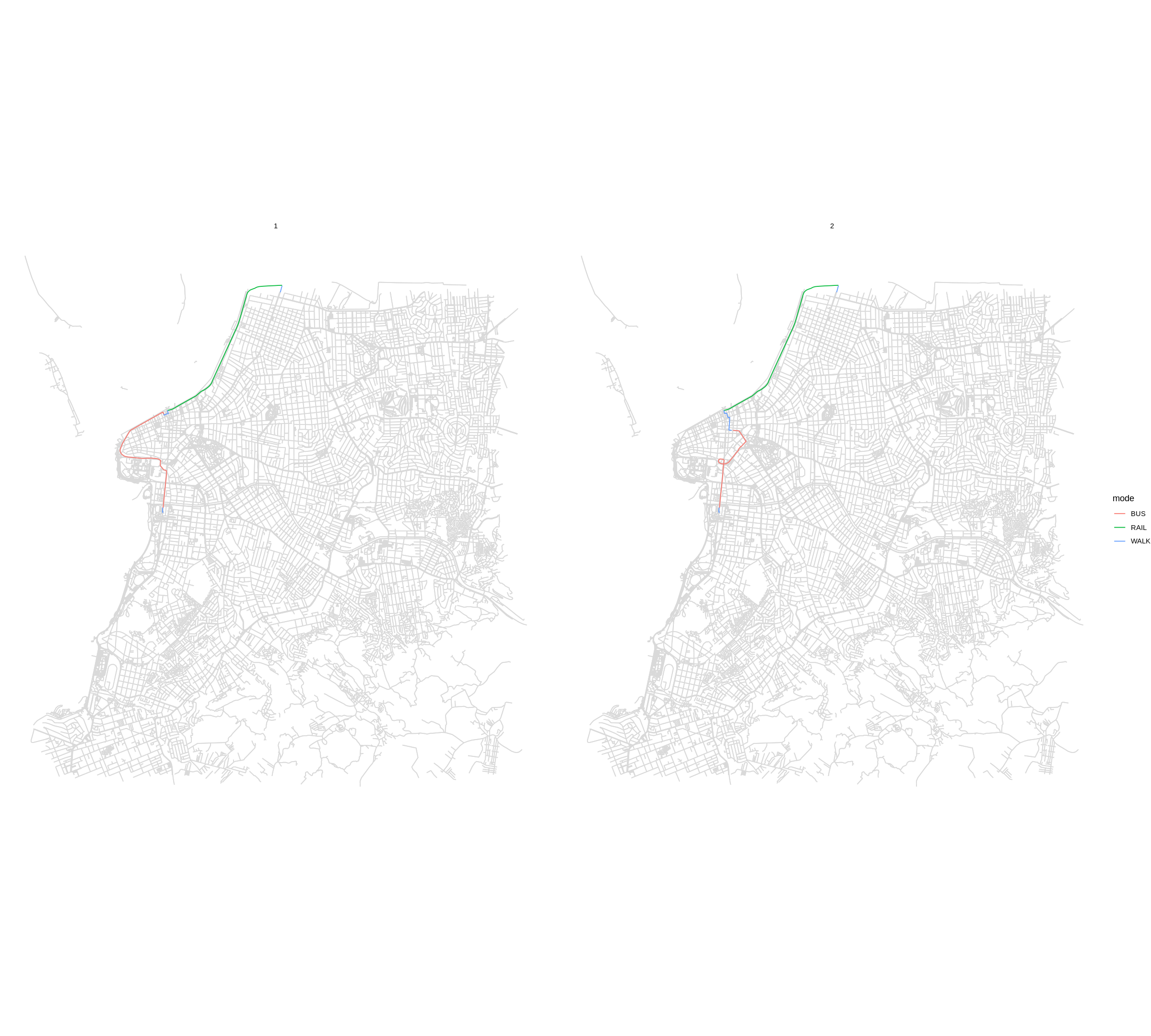
The output is a data.frame sf object, so we can easily visualize the results.

Visualize results

Static visualization with ggplot2 package: To provide a geographic context for the visualization of the results in ggplot2, you can also use the street_network_to_sf() function to extract the OSM street network used in the routing.

# Increase the size of the plot
options(repr.plot.width = 20, repr.plot.height = 18)

# extract OSM network
street_net <- street_network_to_sf(r5r_core)
# extract public transport network
transit_net <- transit_network_to_sf(r5r_core)
# plot
ggplot() +
  geom_sf(data = street_net$edges, color='gray85') +
  geom_sf(data = det, aes(color=mode)) +
  facet_wrap(.~option) + 
  theme_void()

Cleaning up after usage

r5r objects are still allocated to any amount of memory previously set after they are done with their calculations. In order to remove an existing r5r object and reallocate the memory it had been using, we use the stop_r5 function followed by a call to Java’s garbage collector, as follows:

r5r::stop_r5(r5r_core)
rJava::.jgc(R.gc = TRUE)

r5r_core has been successfully stopped.

If you have any suggestions or want to report an error, please visit the package GitHub page.

Where to go next?

• Read r5r documentation for much more details about how to use the library

• Read further examples how to use r5r for spatial accessibility analyses:

  • How to calculate and visualize accessibility in R?

  • How to do route planning using the detailed_itineraries() function?

  • How to configure and use custom fare rules in order to account for monetary travel costs when generating travel time matrices and accessibility estimates?

  • How to calculate and visualize isochrones in R?

  • How to use the pareto_frontier() function to examine the trade-offs between travel time and monetary cost in travel time matrices in r5r?